Book Appointment Now

A practical PCB signal integrity framework: termination, length matching, crosstalk levers, return paths, stackup templates and via optimization.
PCB Signal Integrity: A Practical Framework from Stackup to Routing
Signal integrity is the discipline of making a waveform arrive at its receiver looking the way it left the driver — same amplitude, same timing, same edge shape. Below roughly 50 MHz it mostly takes care of itself; above it, every trace becomes a transmission line and every discontinuity becomes a reflection. Most of what goes wrong — ringing, overshoot, bit errors, failed EMC runs — traces back to a handful of physical causes that can be engineered out systematically.
This guide is the connecting framework for the topic: reflections and their terminations, timing and length matching, the crosstalk levers in order of effectiveness, the return-path rules that decide your EMI performance, stackup templates for 4, 6 and 8 layers, and via optimization. Where a subject deserves its own depth — crosstalk, stackup rules, impedance measurement — the dedicated guides are linked inline.
Table of Contents
- What Signal Integrity Means and When It Starts to Matter
- Reflections: Impedance Discontinuities and Termination Choices
- Timing Budgets: Propagation Delay and Length Matching
- Crosstalk: The Control Levers in Order of Power
- Return Paths and Emissions: The EMI Side of Signal Integrity
- Stackup Templates: 4, 6 and 8 Layers Compared
- Via Optimization: Drill Size, Stub Length and Antipads
- The Design Flow: From Constraints to Verified Layout
- FAQ
- Bringing a High-Speed Design to Fabrication?
What Signal Integrity Means and When It Starts to Matter
The transition from ‘just copper’ to ‘transmission line’ happens when the signal’s edge is faster than the round-trip time of the trace. Practically, that boundary sits somewhere between 50 and 100 MHz clocks or the first gigabit-class serial link. Past it, the interconnect behaves as a distributed network with its own characteristic impedance, and three failure families emerge:
- Amplitude distortion — reflections, ringing, overshoot and undershoot from impedance discontinuities along the path.
- Timing distortion — skew between related signals, jitter from noise, and crosstalk-induced edge shifts that eat setup and hold margins.
- Radiated emissions — loop areas and common-mode currents turning the board into an unintentional antenna, failing CISPR/FCC limits.
The useful insight is that the three families share root causes. A trace routed over a continuous reference plane with controlled impedance simultaneously fixes reflections, crosstalk and emissions. That is why signal integrity work concentrates so heavily on stackup and reference-plane discipline before any trace is routed.
Reflections: Impedance Discontinuities and Termination Choices
A reflection happens whenever a propagating wave meets a change in the impedance it sees — a width change, a via, a connector, or a load that does not match the line. The reflection coefficient Γ = (ZL − Z0)/(ZL + Z0) quantifies it: matched loads reflect nothing; open or shorted ends reflect everything. The engineering task is to shrink Γ at every point along the path and terminate what remains.
| Termination scheme | How it works | Best for | Trade-off |
|---|---|---|---|
| Series (source) termination | Resistor at the driver, roughly Z0 minus driver output impedance | Point-to-point CMOS links — the default for most digital nets | Slightly slower edge at the receiver |
| Parallel termination | Resistor to ground (or rail) at the receiver, value = Z0 | Multi-load buses, fast nets where edge speed is precious | Continuous DC power drain |
| Thévenin (split) termination | Resistor divider setting both match and logic level | Buses needing level setting plus matching | Two resistors per net; rail loading |
| AC termination | Series capacitor into a parallel resistor | Clocks and nets where DC drain is unacceptable | Capacitor selection is frequency-critical; layout area |
The discontinuities between terminations matter as much as the terminations themselves: a 12 mil via stub on a 10 Gbps net is an electrical stub that resonates; changing to a smaller drill, or back-drilling the stub, removes the resonance rather than tuning around it — the dedicated mechanics are in our back-drilling guide.
Timing Budgets: Propagation Delay and Length Matching
Propagation delay through a laminate is set by the effective dielectric constant — for common FR-4 systems, roughly 5.4 ps per millimeter, and slower on high-Dk materials. Timing skew between related signals accumulates from three sources: unequal trace lengths, clock jitter, and crosstalk-induced edge shifts. The classic consumer of margin is the memory interface, where dozens of signals must arrive within fractions of the bit period.
- Length matching. DDR-class buses typically hold intra-group matching to a few mils; the tolerance comes from the timing budget, not from a universal rule — derive it per interface.
- Serpentine discipline. Tuning serpents must keep amplitude spacing of 2–3× trace width so the meanders do not couple to themselves.
- Worst-case analysis. Simulate timing at the slow/fast process corners, voltage extremes and temperature ends — a design that closes only at nominal conditions is not closed.
- Match the reference, not just the length. Signals propagating over different dielectric heights (microstrip vs stripline) run at different speeds; equal physical length does not equal equal delay.
This last point is a stackup issue in disguise: mixed-layer routing within one bus complicates delay matching. Keeping a bus on one layer pair simplifies the budget — one of the stackup principles detailed in our stackup design guide.
Crosstalk: The Control Levers in Order of Power
Crosstalk is capacitive plus inductive coupling between neighbors, and its control levers are not equally effective. Ordered by payoff:
- 1. Dielectric height. Coupling falls steeply as the trace hugs its reference plane; thin dielectric is the strongest structural lever, set at stackup time.
- 2. Spacing. The 3W rule (center-to-center spacing ≥ 3× trace width) is the standard first-order guard for parallel runs.
- 3. Parallel length. Coupling accumulates over the parallel run; orthogonal routing on adjacent layers and staggered breakouts shrink it for free.
- 4. Edge rate. Slowing a driver (series resistor, or a slower part) removes harmonic content — effective, but only where timing allows.
- 5. Guard traces. Grounded guards with stitching vias help sensitive nets like clocks and resets; without frequent grounding they can do more harm than good.
- 6. Differential signaling. Moving critical links to differential pairs buys common-mode rejection and crosstalk immunity measured in tens of dB.
The full quantitative treatment — near-end versus far-end coupling, the spacing curves, and the fixes per topology — lives in our crosstalk causes and fixes guide, which pairs with this section as the deep dive.
Return Paths and Emissions: The EMI Side of Signal Integrity
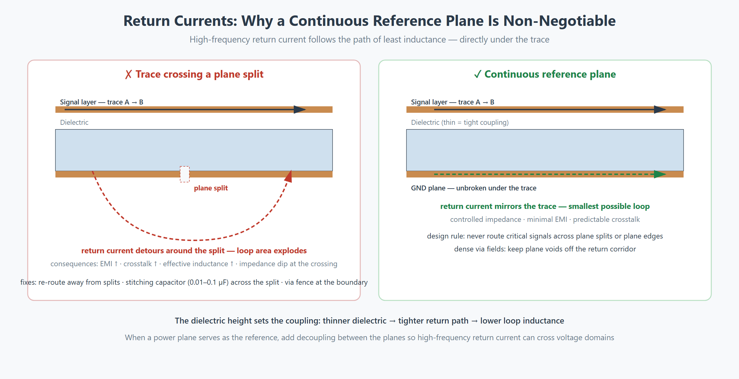
Every signal current returns to its source, and at high frequency the return chooses the path of least inductance — the mirror image of the trace on the reference plane directly beneath it. Signal integrity and EMC meet exactly here: a trace whose return path is interrupted does not just radiate, it also reflects and couples worse. The two failure pictures in the diagram above cover most field cases:
- Plane splits. A trace crossing a gap in its reference plane forces the return to detour; the enlarged loop radiates and couples. Fix by routing away from splits, adding a stitching capacitor across the split, or via-fencing the boundary.
- Layer transitions. A signal changing reference layers needs its return to follow; add a ground via beside the signal via, or reference the same plane family on both layers.
- Via anti-pad fields. Dense via clusters punch holes in the reference corridor; keep the return lane continuous under critical nets.
- Power-plane references. Referencing a power plane is legal with decoupling between the planes so high-frequency return current can cross the voltage boundary.
Loop-area discipline extends to the power distribution network: decoupling capacitors placed so that every IC sees a tight capacitor loop, with multiple values covering kHz-to-GHz, keep the PDN quiet — and a quiet PDN radiates less. The mechanism is the same one behind board-edge stitching and via fences: give the currents a designed path so they never invent one.
Stackup Templates: 4, 6 and 8 Layers Compared
Three working templates cover most signal-integrity-driven builds. The comparison assumes standard FR-4 systems; the layer-count economics against lower counts are in our 2-layer vs 4-layer comparison:
| Template | Layer order (top → bottom) | Signal layers with adjacent reference | Character |
|---|---|---|---|
| 4-layer standard | Signal — GND — PWR — Signal | 2 of 2 | Every signal layer referenced; limited routing density; the entry point for controlled impedance |
| 6-layer optimized | Signal — GND — Signal — PWR — Signal — Signal | 4 of 4 (two layers plane-adjacent on both sides) | The volume workhorse: full referencing with two extra routing layers |
| 8-layer high-performance | Signal — GND — Signal — Signal — PWR — Signal — GND — Signal | 6 of 6, with two stripline layers double-referenced | High density plus EMI headroom; the internal signal pair is shielded on both sides |
Reading the table by its third column explains the whole game: a signal layer is only as good as its reference. The 6-layer template’s value is that all four signal layers touch a plane; the 8-layer template buys two stripline layers — fully enclosed between planes — which are the quietest routing real estate on any board. Symmetry across the board centerline (balanced copper and dielectric) keeps the stack flat and manufacturable; the full rule set is in the stackup guide.
Via Optimization: Drill Size, Stub Length and Antipads
Vias are mandatory and inductive — the goal is to make each one small, short and consistent:
- Drill size. A ~0.2 mm mechanical via carries noticeably less parasitic inductance than a 0.3 mm one; HDI microvias shrink it further — the capability ladder is in our HDI vs standard PCB guide.
- Stub removal. The unused barrel beyond the last connected layer resonates; back-drilling removes it, and the length budget that matters is the residual stub — covered with numbers in the back-drilling guide.
- Antipad sizing. The clearance around a via in its reference plane sets the local capacitance; oversized antipads create impedance bumps, undersized ones add loading. Differential pairs need identical antipads on both legs.
- Transition discipline. High-speed nets should change reference layers as rarely as possible, and every transition that must happen gets its return via next to it.
For impedance targets, the routine conversation is 50 Ω single-ended and 90–100 Ω differential, held within ±10% standard tolerance (±5% where the link demands it) — how those numbers are measured and reported is the subject of our impedance measurement guide.
The Design Flow: From Constraints to Verified Layout
Signal integrity results come from process, not heroics. The working flow:
- Plan. Classify nets by speed and sensitivity; decide topologies; agree the stackup and impedance targets with the fabricator before layout starts.
- Constrain. Encode the rules — length matching, spacing, reference-plane corridors, via budgets — into the CAD constraint system so the rules survive team handoffs.
- Route by priority. Clocks and differential pairs first with their returns, then buses, then the low-speed fill; guard and stitching structures go in with the nets they protect, not as an afterthought.
- Verify. Post-layout extraction and simulation on the critical nets, PDN analysis on the power tree, and a DRC pass that includes the electrical rules — a clean geometric DRC says nothing about a return path crossing a split.
- Hand off. Complete fabrication data with impedance requirements and stackup tables explicit; the Gerber handoff format itself is standardized by UCamco’s Gerber specification, and the review checklist for what the fabricator needs is in our DFM analysis guide.
Materials sit underneath every step: as data rates climb past 10 Gbps, loss tangent becomes the selector, and the laminate decision framework — Dk stability, Df tiers, glass-style effects — is laid out in our high-frequency materials guide.
Frequently Asked Questions
At what speeds does signal integrity start to matter?
The practical boundary is where the edge becomes faster than the trace’s round-trip time — typically clock rates from 50–100 MHz or the first gigabit-class serial link. Below that, most nets behave as lumped circuits; above it, every interconnect is a transmission line and impedance control becomes mandatory.
What is the best termination scheme for a point-to-point CMOS net?
Series (source) termination: a resistor at the driver sized to bring the total source impedance up to the line impedance. It absorbs the reflection with zero DC power drain, at the cost of a slightly slower edge at the receiver — acceptable for most point-to-point digital links.
Why is a trace crossing a plane split a problem?
The high-frequency return current must mirror the trace on its reference plane. A split forces the return to detour around the gap, enlarging the loop — which increases inductance, radiates EMI, increases crosstalk, and creates a local impedance disturbance. Fixes are re-routing, a stitching capacitor across the split, or a via fence at the boundary.
Does the 3W rule eliminate crosstalk?
No — it is a first-order guard that keeps coupling small for parallel runs. The stronger levers are dielectric height (set in the stackup) and shorter parallel length. 3W spacing combined with a thin dielectric and modest parallel runs is the realistic working recipe; guard traces are reserved for genuinely sensitive nets like clocks.
Should length matching be done in physical length or delay?
Delay. Signals on microstrip and stripline layers propagate at different speeds for the same physical length, so a bus routed across both needs delay-based matching or a per-layer length factor. Keeping a bus on one layer pair avoids the complication entirely.
When is back-drilling worth requiring?
When stub length becomes a meaningful fraction of the signal’s wavelength — typically multi-gigabit links through thick boards with high layer counts. The residual stub after back-drilling is specified in the fabrication drawing; the technique, limits and cost logic are detailed in the back-drilling guide.
Why does the 8-layer template outperform two 4-layer boards of the same size?
Layer quality, not just count: the 8-layer template provides two stripline layers fully enclosed between planes — the quietest routing environment available — plus four more plane-referenced signal layers. Two separate 4-layer boards cannot offer that shielding or the inter-layer routing freedom.
What impedance tolerances are standard?
±10% is the standard control for single-ended 50 Ω and differential 90–100 Ω designs, with ±5% available where high-speed links demand it — feasibility is confirmed against the actual stackup during engineering review, and compliance is verified on the production coupon.
Bringing a High-Speed Design to Fabrication?
Send your stackup plan, impedance targets and the net classes that worry you, and our engineering team will confirm the layer structure, controlled-impedance feasibility and back-drill options before layout freezes. Production runs from 2 to 30 layers (up to 64 layers for prototypes, subject to per-order review), with process feedback typically the same day.
Season PCB direct: Tel (+86) 18681528532 | WhatsApp +86 18681528532
E-mail: roc@season-pcb.com