Book Appointment Now

Practical PCB signal trace design rules: path planning, differential pairs, impedance against the pressed stack, return paths, spacing and handover data.
PCB Signal Trace Design: Routing Rules That Hold Up in Production
Most PCB signal trace design advice is written for the simulator and stops at the factory gate. The trace that behaves in the field solver is not the trace that comes off the etch line: copper is trapezoidal, dielectric heights move when the panel is pressed, and the coupon – not the model – decides whether the board ships. This article starts from the geometry a fabricator can actually hold and works back to the rules you should route by.
The focus is on the decisions that change a layout: what trace width and spacing really buy you, when a differential pair should be tightly or loosely coupled, why the return path matters more than the trace, and which limits are process limits rather than physics. Where a rule is a manufacturing constraint rather than a signal integrity law, it is labelled as such, because that distinction is what stops a redesign two weeks before build.
Table of Contents
- Where Signal Trace Design Actually Starts
- Path Planning: Length, Corners and What the Etch Process Does
- Differential Pairs: Coupling, Spacing and Length Matching
- Controlled Impedance in PCB Signal Trace Design
- Reference Planes and the Return Path
- Layer Transitions, Vias and Stubs
- Crosstalk and EMI: Spacing Rules That Actually Work
- Manufacturing Limits Behind PCB Signal Trace Design
- Verification: What Proves the Trace Was Built Right
- Handover Checklist for PCB Signal Trace Design
- FAQ
- Get Your Trace Geometry Checked Before Release
Where Signal Trace Design Actually Starts
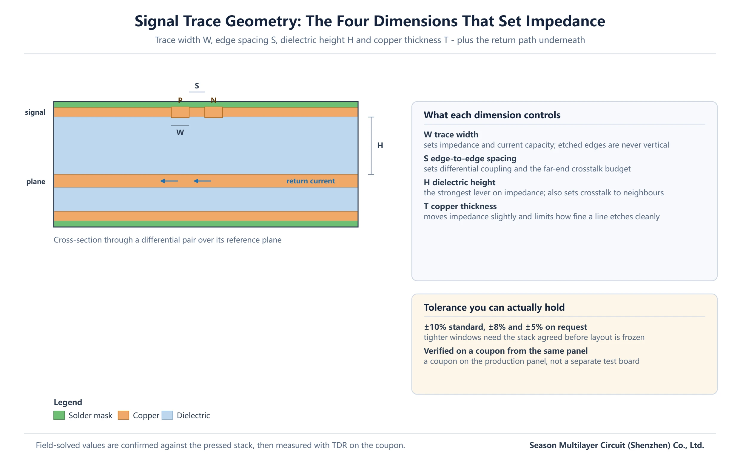
A trace is not a line on a drawing; it is a copper cross-section sitting at a measured distance from a plane. Four numbers define it: the width at the top of the copper, the width at the base after etching, the height of the dielectric to the nearest reference plane, and the thickness of the copper itself. Everything that follows – impedance, loss, crosstalk, current capacity – falls out of those four and the dielectric constant of the material around them.
The first practical consequence is that the stack, not the schematic, sets the rules. Until the layer order and the dielectric heights are fixed, a trace width is a guess. That is why the ordering of decisions matters: agree the stackup and the reference planes first, derive the widths second, and only then route. Designers who route first and ask for impedance afterwards are the ones who get asked to move copper weights, as described in our note on PCB stackup design.
The second consequence is that every number has a tolerance. Copper thickness varies across a panel, dielectric height varies with resin flow, and the etched edge is never vertical. Routing to a nominal value with no margin is routing to a board that will be retuned in CAM.
Path Planning: Length, Corners and What the Etch Process Does
Shorter is better, but not for the reason usually given. Trace length matters because conductor loss and dielectric loss accumulate with distance, and because a longer trace is more likely to cross a discontinuity somewhere along the way. The practical rule is to place the driver near its load, keep the critical nets on the layers closest to their reference plane, and avoid detours that add length without buying clearance.
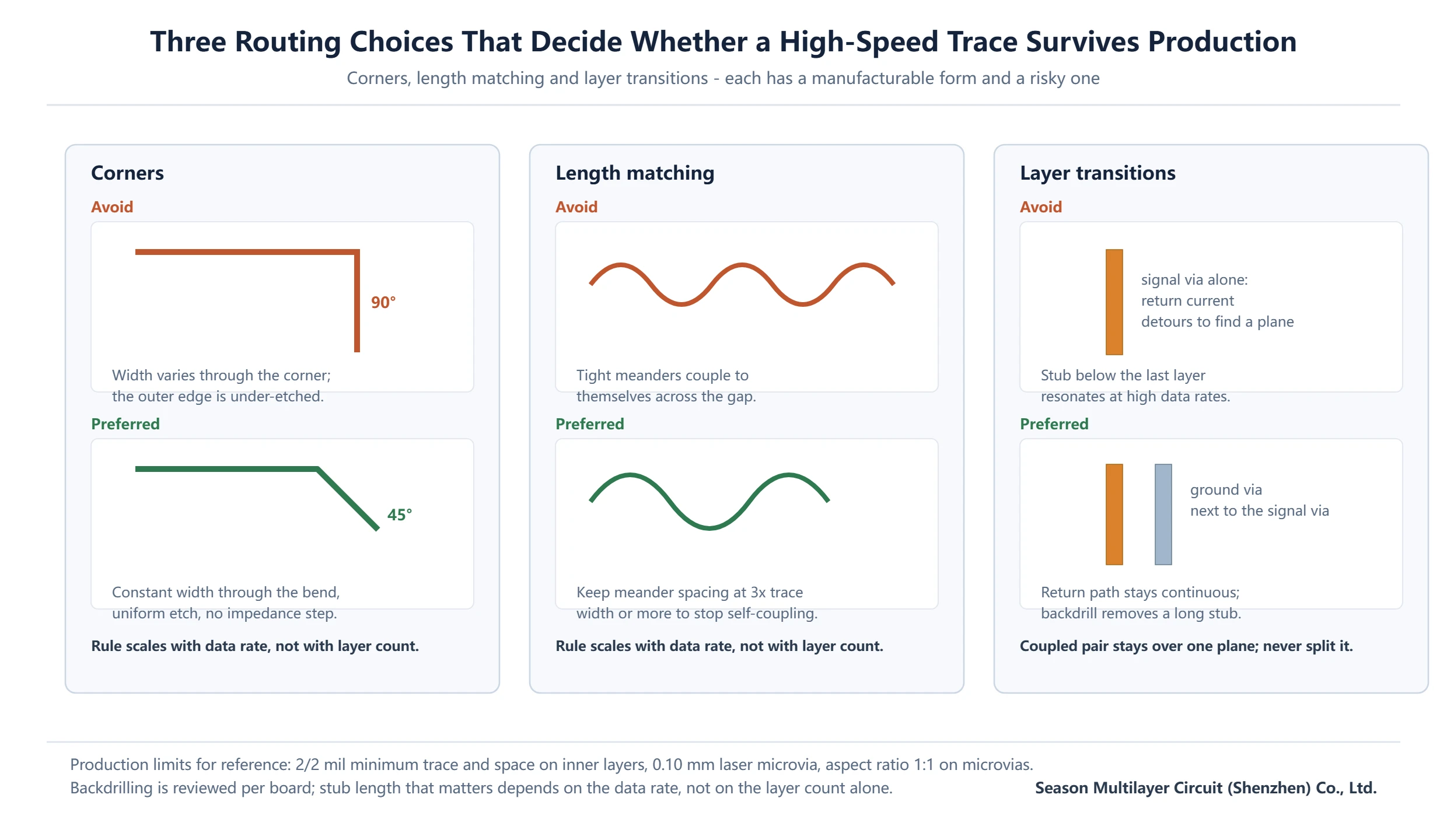
Corners are a smaller signal integrity issue than folklore suggests and a larger manufacturing one. A sharp 90-degree corner on a modern digital board is electrically tolerable at most data rates, but the outer edge of the corner etches differently from the inner edge, so the width is not constant through the bend. Use 45-degree or curved corners: they hold width, they etch uniformly, and they remove an argument at inspection.
- Route critical nets on layers adjacent to a solid plane, never across a plane split
- Keep 45-degree or arc corners on any net with an impedance requirement
- Avoid routing over gaps, cut-outs and antipads in the reference plane
- Leave the last 3 to 5 mm of a pad entry straight so the neck-down is consistent
- Do not route a controlled-impedance net on the outer layer under a solder mask discontinuity you have not modelled
Differential Pairs: Coupling, Spacing and Length Matching
A differential pair carries the signal in the difference between two traces and returns very little current through the plane, which is what makes it tolerant of noise. The design choice is how tightly to couple the two halves. Tight coupling – narrow edge-to-edge spacing – makes the pair less sensitive to the plane distance and to external aggressors, and it reduces the loop area. Loose coupling gives a wider trace for the same differential impedance, which lowers conductor loss.
| Coupling choice | What it improves | What it costs |
|---|---|---|
| Tight (spacing near trace width) | Common-mode rejection, smaller loop, less sensitivity to plane distance | Narrower traces, higher conductor loss, tighter etch tolerance |
| Loose (spacing 2x to 3x width) | Wider traces, lower loss, easier to manufacture | Larger loop, more sensitivity to the reference plane |
| Broadside (stacked on adjacent layers) | Very tight coupling, compact routing | Layer-to-layer skew from dielectric variation between the two layers |
Length matching is where most layouts lose yield unnecessarily. Match the two halves of a pair to each other at the point where the skew budget actually applies – usually at the receiver – and keep the meander geometry sane: segment lengths at least three times the trace width apart, so the serpentine does not couple to itself. Matching every net in a bus to the longest one instead of to a common target is a common way to add length, loss and crosstalk for no benefit.
One manufacturing note: the pair has to stay over one plane for its whole run. If the reference changes underneath a differential pair, the return current has to find a new path, and the discontinuity shows up as a common-mode conversion that no amount of length matching will fix.
Controlled Impedance in PCB Signal Trace Design
Impedance control is a contract between three parties: the designer who specifies a target and a tolerance, the fabricator who sets the pressed dielectric height and the trace width, and the coupon that proves the result. Nominal dielectric heights in a stackup drawing describe the material before pressing. Once resin flows and copper fills the neighbouring layer, the actual height is different, and the width has to be recalculated against that number. This is why a fabricator will come back with proposed widths even when the layout looks complete.
| Target | Typical geometry driver | Practical note |
|---|---|---|
| 50 ohm single-ended | Width relative to dielectric height to the plane | The most forgiving target; standard tolerance usually sufficient |
| 90 ohm differential | Width plus edge spacing, tightly or loosely coupled | State the coupling assumption with the target |
| 100 ohm differential | Slightly looser coupling or wider spacing than 90 ohm | Confirm the receiver tolerance before choosing |
| 75 ohm / RF nets | Often needs a specific dielectric height | May force a stackup change rather than a width change |
On tolerance, ±10% is the standard offer, and ±8% or ±5% are available when the stack, copper weights and coupon design are agreed before layout is frozen. Tighter windows are not free: they reduce the process window and can lower yield, so specify them where the interface needs them rather than across the whole board. Measurement is done with TDR on a coupon built on the production panel, which our article on impedance measurement methods covers in detail.
Reference Planes and the Return Path
Current flows in a loop. The forward path is the trace; the return path is the plane underneath it, and at high edge rates the return current crowds directly beneath the trace whether or not the schematic shows a connection there. Everything that interrupts that path – a split, a gap, a row of antipads, a layer change without a nearby return via – forces the current to detour, and the detour is what radiates and what couples into neighbours.
This makes plane continuity a routing rule, not a layout preference. Keep at least one solid plane adjacent to every high-speed layer across the whole board. If a plane must be split for isolation, no controlled-impedance trace may cross the split; route around it, or change the layer order so the trace has an uninterrupted reference. Where a trace has to change layers, place a ground via within a fraction of a millimetre of the signal via so the return current has somewhere to go.
Stitching vias around plane edges, connector shells and board perimeters are cheap insurance. They shorten the return path for any current that does stray, and they cost nothing in routing area if they are placed during layout rather than added afterwards.
Layer Transitions, Vias and Stubs
Every layer change adds a discontinuity: the via has its own capacitance and inductance, and the portion of the barrel that carries no signal – the stub – resonates at a frequency set by its length. At moderate data rates a stub is invisible. At the rates used on modern serial links it acts as a notch filter in the channel, which is why backdrilling exists. The rule is proportional: the faster the edge, the shorter the tolerable stub.
Via size is a process decision as much as an electrical one. A smaller via has less capacitance and a smaller antipad, which frees routing area, but it is harder to plate reliably and it constrains the aspect ratio. On HDI builds the laser microvia is 0.10 mm as standard, with 0.076 mm available after review, held at roughly a 1:1 aspect ratio; on through-hole builds the mechanical drill is typically 0.20 mm minimum. Where a long stub has to go, backdrilling removes the unused barrel and is reviewed per board, not assumed.
For the layer change itself, two habits pay off: keep the paired signal and its return via close together, and avoid changing layers in the middle of a length-matched segment, because the via delay has to be included in the match.
Crosstalk and EMI: Spacing Rules That Actually Work
Crosstalk falls off quickly with spacing and slowly with length. Doubling the edge-to-edge spacing between two traces cuts the coupled noise by a large factor; halving the parallel run length cuts it roughly in half. When a board has a crosstalk problem, the cheapest fix is almost always to shorten the parallel run or to move one net to a layer with a plane between it and the aggressor – not to add spacing everywhere and lose routing density.
| Rule of thumb | Where it applies | Why it works |
|---|---|---|
| 3x trace width spacing (3W) | Between unrelated nets on the same layer | Puts most of the fringe field inside the spacing |
| Keep plane between aggressor and victim | Adjacent signal layers | A solid plane between layers is far stronger than spacing |
| Shorten parallel runs | Long buses routed side by side | Coupled energy accumulates with parallel length |
| Guard traces with stitching vias | Very sensitive analogue or clock nets | Gives the coupled field a low-impedance destination |
| Separate analogue and digital returns | Mixed-signal boards | Stops shared impedance turning into noise |
On EMI, the usual suspects are not the traces but the discontinuities: a return path forced around a split, a cable shield bonded at one end, a connector whose pinout puts a signal next to a return pin that is not there. Fix the loops before adding shielding, because a shield over a bad return path moves the problem rather than removing it.
Manufacturing Limits Behind PCB Signal Trace Design
Some of what looks like a signal integrity limit is really a process limit, and knowing which is which saves a lot of argument. Minimum trace and space on inner layers is 2/2 mil as standard, with 1.8/1.8 mil achievable on samples after review; finer geometries raise the etch tolerance problem described earlier and usually force thinner copper. Laser microvias are 0.10 mm standard, 0.076 mm on review, at about 1:1 aspect ratio. Layer counts run from 2 to 30, and every additional HDI stage typically adds 30% to 100% to the board cost because the press, drill, plate and image cycle is repeated.
Etch compensation is the other process reality. Artwork is drawn deliberately wider or narrower than the finished target so the etch lands on the number, and the allowance depends on copper weight. A 1 oz inner layer needs a bigger allowance and ends up with a more trapezoidal edge than a 0.5 oz layer, which is one reason a fabricator may propose changing inner copper weight when impedance targets are tight.
Material choice sits underneath all of this. Dielectric constant sets the width for a given impedance and the propagation delay; dissipation factor sets the loss at high frequency. Our laminate and materials guide lists the grades we hold, and the wider design consequences are covered in high-speed PCB design rules.
Verification: What Proves the Trace Was Built Right
Verification has three layers, and they answer different questions. Electrical test asks whether the nets are connected as drawn. The impedance coupon asks whether the geometry came out as calculated. Inspection against IPC-6012 asks whether the construction is acceptable. A board can pass any one of the three and still fail the others, so ask for all three on a controlled-impedance build.
- Netlist comparison and electrical test – flying probe for prototypes, a fixture for volume
- Impedance measured with TDR on a coupon from the production panel, reported against the specified tolerance
- Dimensional and microsection checks where the stack is tight – dielectric heights and copper thickness measured, not assumed
- Visual and dimensional acceptance against IPC-6012 Class 2, or Class 3 where the application requires it
The acceptance criteria themselves are published by the Global Electronics Association standards programme, and the practical reading of them is covered in our PCB manufacturing services overview. Ask for the impedance report with the shipment, not after a failure – it is the one document that tells you whether the process held on your specific panel.
Handover Checklist for PCB Signal Trace Design
Most impedance problems on a first build trace back to a missing line in the data package rather than to a bad calculation. The list below is what a fabricator needs in order to return buildable widths instead of questions. Where a decision is still open, send it as a question; a stated unknown is much cheaper than a silent assumption that becomes a respin.
| Handover item | What it decides | Typical content |
|---|---|---|
| Stackup with dielectric heights | Trace width for every impedance target | Layer order, material, height per dielectric |
| Impedance table | Width, spacing, tolerance class and coupon | Target, tolerance, layers, nets, coupling assumption |
| Copper weights per layer | Etch allowance and achievable line width | Outer and inner weights, plane layers included |
| Differential pair definitions | Which nets are matched, and to what skew | Net pairs, match point, skew budget |
| Via and via-in-pad plan | Drill sizes, aspect ratio, fill requirements | Via types, sizes, backdrill where needed |
| Acceptance class and reports | Inspection criteria and documents shipped | IPC class, electrical test, impedance report |
Fabrication data itself should be clean Gerber data with an unambiguous drill chart and a readme that states the finished board thickness, the surface finish and the impedance requirements in one place. For a reference build at this density, the 12-layer high-speed backplane page shows how the stackup and impedance targets were documented before release.
Frequently Asked Questions
What is the most important rule in PCB signal trace design?
Keep every controlled-impedance trace adjacent to a solid reference plane for its entire run. Most signal integrity failures trace back to a return path that was interrupted by a split, a gap or a layer change with no nearby return via, rather than to a wrong trace width.
How much spacing do I need between signal traces?
Three times the trace width is a workable default for unrelated nets on the same layer. Shortening the parallel run is usually more effective than adding spacing, and putting a solid plane between two signal layers is far stronger than either.
Do 90-degree corners really cause problems?
Electrically they are tolerable at most modern data rates. The reason to avoid them is manufacturing: the outer edge of a sharp corner etches differently from the inner edge, so the width is not constant through the bend. Use 45-degree or curved corners.
Should differential pairs be tightly or loosely coupled?
Tight coupling improves common-mode rejection and reduces sensitivity to the reference plane distance, at the cost of narrower traces and higher conductor loss. Loose coupling gives wider traces and lower loss but a larger loop. State which you assumed when you specify the impedance target.
What impedance tolerance should I specify?
±10% is standard and covers most designs. ±8% and ±5% are available when the stackup, copper weights and coupon design are agreed before layout is frozen. Tighter windows reduce the process window and can lower yield, so apply them where the interface needs them.
When does a via stub start to matter?
When the stub length becomes a meaningful fraction of the wavelength of the signal’s edge rate – at higher data rates on serial links, a long unused barrel acts as a notch in the channel. Backdrilling removes it and is reviewed per board rather than applied by default.
How is controlled impedance actually verified?
With TDR on a coupon produced on the same production panel, measured against the tolerance you specified. Electrical test confirms connectivity and IPC-6012 inspection confirms construction, but only the coupon report tells you whether the geometry came out as calculated.
Get Your Trace Geometry Checked Before Release
Send the layout with your stackup, copper weights and impedance table, and the engineering review will return the widths we can hold on the pressed stack, together with any deviation we would propose and why. Nothing is released without your approval.
We build from 2 to 30 layers with 2/2 mil minimum trace and space on inner layers, laser microvias from 0.10 mm, and impedance control at ±10%, ±8% or ±5% depending on the stack agreed at review.